
Bridging Theory and Expert Judgment: Advances in Polarization Metrics and Their Empirical Correlations
In our investigation of opinion divergence dynamics, we conducted a comprehensive experimental study that bridges theoretical models with expert evaluation. Our objective was to elucidate the relationships among various polarization measures and to assess their alignment with expert judgment. I personally carried out all the experiments and authored this article as a means of both disseminating our findings and maintaining a detailed record for future reference. It is important to note, however, that this work is the result of a collaborative effort by the polarization measures team from the Promueva group, which includes Frank D. Valencia, Juan Francisco Díaz, Jesús Aranda, and Carlos Pinzón. Each of these team members has significantly contributed to guiding the experimental process, providing critical feedback and advice that have shaped the direction of this project. I am truly grateful for the opportunity to work alongside such dedicated colleagues.
We begin by formally defining a polarization measure as a function , where for any consensus distribution , we have , and for any extremal distribution , we have for all . Here, denotes the set of all opinion distributions. An opinion distribution is defined as a function with finite, non-empty support . For each opinion value , represents its associated weight, and the total mass of is defined as
For notational clarity, we represent an opinion distribution as an ordered pair
where and . This representation uniquely characterizes the opinion distribution through for each , with total mass .
To analyze the correlation between various polarization measures from the literature (implemented in our package), we constructed an experimental framework examining all possible opinion distributions corresponding to a population of size distributed across bins, representing a Likert scale. The generation of these distributions employed the classical Stars and Bars combinatorial method: for any pair of positive integers and , the number of -tuples of non-negative integers summing to is given by
corresponding to the weak compositions of . For fixed , this sequence appears along the st diagonal of Pascal's triangle.
In our analysis of these polarization measures, we examined their inter-correlations using Kendall's tau-b coefficient. Notably, since all measures under consideration satisfy a symmetry property where mirror images defined by are equivalent, we reduced our analysis from 4,598,126 to 2,299,063 unique distributions. The Kendall tau-b coefficient, introduced by Kendall (1945), was specifically chosen for its ability to handle ties in ranking data.
where represents the number of concordant pairs, the number of discordant pairs, and , account for ties in the first and second quantity respectively. Two pairs of observations and are considered concordant if both and , or if both and . Conversely, they are discordant if and , or if and .
This coefficient provides several advantages over other correlation measures. First, it is robust to outliers since it depends only on the relative ordering of values rather than their magnitudes. Second, it explicitly accounts for ties in the data through the terms and , making it particularly suitable for ordinal data or data with repeated values. Third, it has a clear probabilistic interpretation: represents the difference between the probability of observing concordant and discordant pairs in the data.
The coefficient ranges from -1 to 1, where 1 indicates perfect positive correlation (the rankings are identical), -1 indicates perfect negative correlation (the rankings are exactly opposite), and 0 indicates no correlation (the rankings are independent). In the context of our analysis, Kendall's tau-b provides a robust way to assess how different polarization measures rank distributions, accounting for the possibility of measures assigning equal polarization values to different distributions.
Correlation Analysis of Polarization Measures
To implement our analysis, we developed the following computational framework:
def main(k: int = 100, n: int = 5):
    calculator = MeasureCalculator()
    total_distributions = count_distributions(k, n)

    for i, (x, weights) in enumerate(generate_distributions(k, n)):
        calculator.process_distribution(x, weights)

    values = calculator.get_values()
    correlation_matrix = compute_kendall_matrix(values)
Our computational analysis revealed several significant patterns in the relationships among polarization measures. Most notably, we confirmed empirically the theoretical equivalence previously demonstrated between and , as both measures exhibit identical behavior across all distributions. Furthermore, our findings align with previous research presented in "A New Opinion Polarization Index Developed by Integrating Expert Judgments" (Frontiers in Psychology, 2021), regarding the diminished effectiveness of the measure when employing high values of the identification parameter .
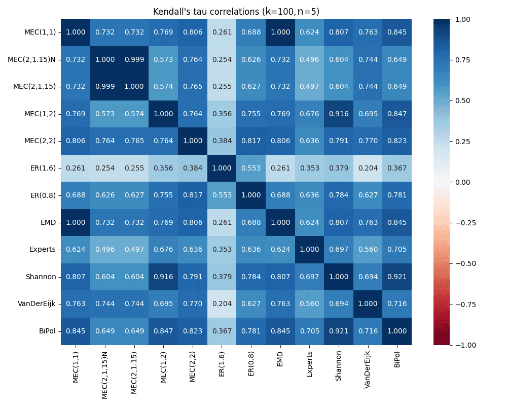
The correlation between and its normalized variant shows an expected near-perfect correlation (), with the negligible difference likely attributable to floating-point arithmetic precision limitations in numerical computations. A particularly notable observation is the strong correlation between and 's polarization measure (). While maximizes the weighted sum of pairwise distances between two disjoint subsets of opinions, 's measure quantifies polarization through the entropy of opinion distances from the mean, both capturing different mathematical aspects of opinion dispersion. The measure shows consistently lower correlations with other measures ( in most cases), indicating it captures fundamentally different aspects of polarization. The expert-based interpolated measure, given by
shows moderate correlations with most measures (), with strongest agreement with () and (). However, this measure exhibits several theoretical shortcomings. Most notably, it yields zero polarization when either extreme pairs or are zero, contradicting basic polarization principles. Such behavior, among other issues, highlights the limitations of direct linear interpolation approaches in capturing the complex nature of opinion polarization.
These findings suggest that 's parameters could potentially be tuned to approximate other polarization measures. Future work could explore this possibility systematically, aiming to find parameter combinations that minimize the distance to target measures while maintaining desirable theoretical properties. Such an investigation could lead to a unified framework where serves as a generalized polarization measure, capable of reproducing various existing indices through appropriate parameter selection.
Expert Validation of Polarization Measures
To validate different polarization measures against expert judgment, we implemented the following analysis framework:
def validate_with_experts():
    # Load expert data and distributions
    data = ValidationData()
    distributions = data.get_normalized_distributions()
    expert_scores = data.expert_scores

    # Calculate polarization values for each measure
    calculator = ValidationCalculator()
    calculator.process_distributions(data.x_values, distributions)
    measure_values = calculator.get_values()

    # Compute Kendall's tau-B correlations with expert scores
    correlations = {}
    for measure_name, values in measure_values.items():
        tau, _ = kendalltau(expert_scores, values)
        correlations[measure_name] = tau
A fundamental aspect in validating polarization measures is their ability to capture expert judgment regarding what constitutes a polarized state of opinions. In this context, a seminal study by Koudenburg et al. (2021) collected evaluations from 60 international experts on polarization for a set of 15 opinion distributions represented as histograms.
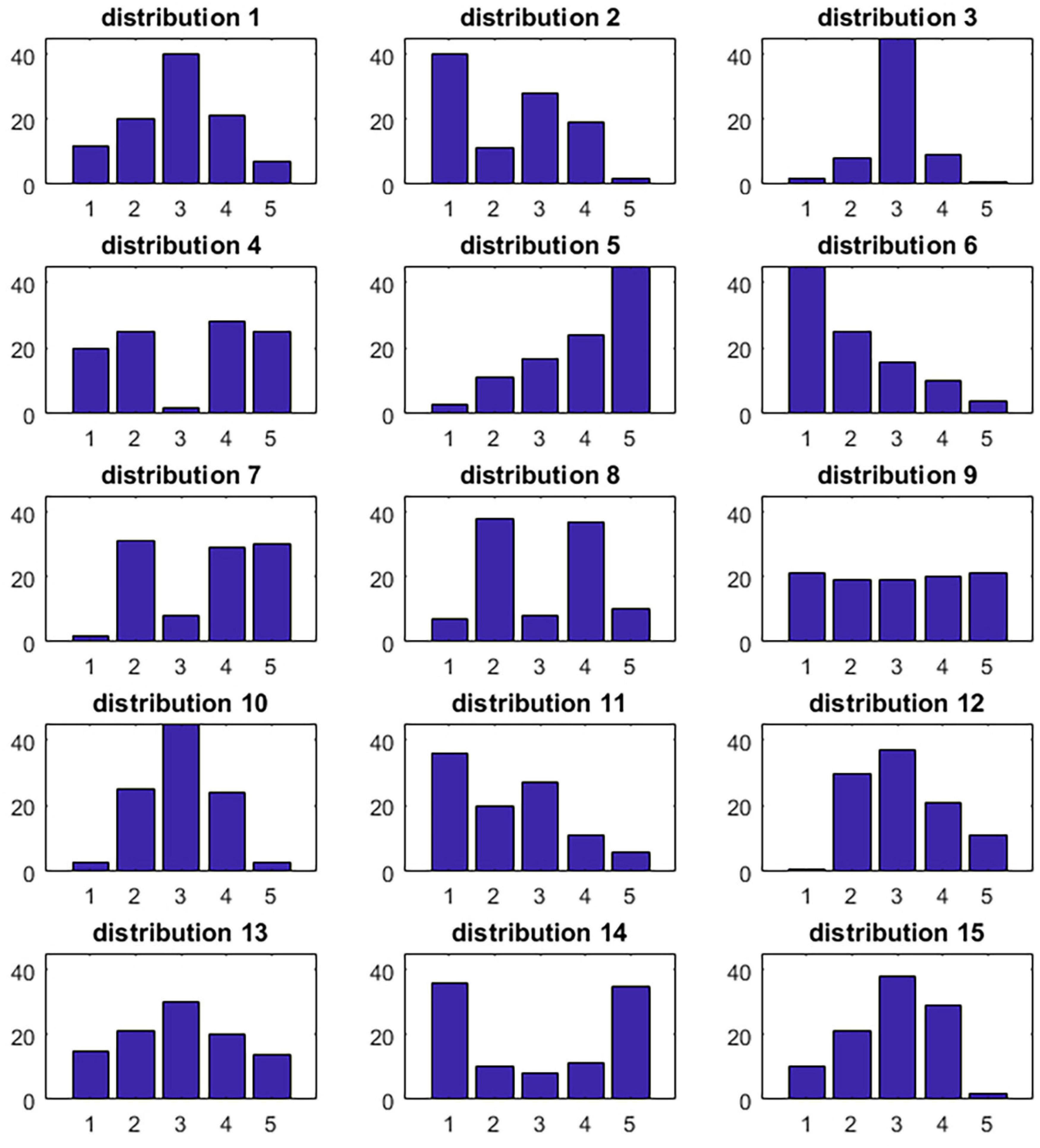
The experts rated each distribution on a scale from 0 (not polarized) to 100 (completely polarized), thereby establishing a reference order to validate different polarization measures. This original order of the histograms reflects the expert consensus on the relative levels of polarization for each distribution. To validate the various polarization measures available in the literature, we compared how each measure would order these same 15 histograms and computed the Kendall between these orders and the original order provided by the experts. This methodology allows us to assess how well each measure captures the expert intuition about polarization.
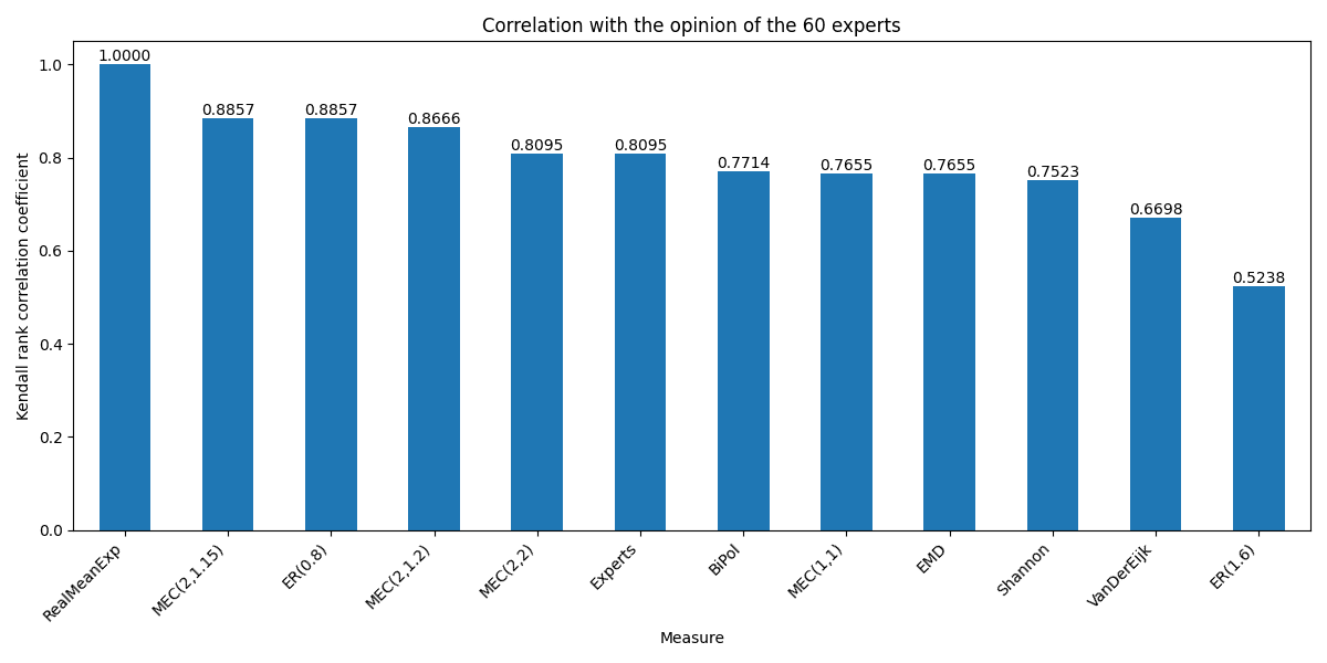
As can be observed in the graph, some measures exhibit a stronger correlation with expert judgment than others. Notably, and with correlations of approximately 0.89. The measure shows a moderate correlation of 0.77, while other measures such as and exhibit lower correlations of 0.67 and 0.52 respectively.
These results suggest that not all polarization measures capture expert intuition equally well regarding what constitutes a polarized state. The differences in correlations reveal the strengths and limitations of each measure in reflecting the specific aspects of polarization that experts consider important. Further research remains to be done to determine the optimal and parameters for , both theoretically and experimentally, that could potentially better align with expert judgment while maintaining desirable mathematical properties.
Axiomatic Foundations and Measure Properties
Having examined the empirical correlations between different polarization measures and explored their alignment with expert judgment, we now turn to a more theoretical analysis of how well existing measures satisfy the fundamental axioms proposed by Esteban and Ray for polarization measurement. These axioms provide a rigorous mathematical framework for evaluating the theoretical soundness of polarization measures and their ability to capture key properties of opinion distributions.
The Esteban-Ray measure represented a breakthrough in the formal measurement of polarization by proposing a theoretically grounded axiomatic framework. Their measure takes the form:
for some constants and where . This measure was characterized by three fundamental axioms that capture key intuitions about what constitutes polarization:
Axiom 1. For any and any , there exist and such that, for any and any with and ,
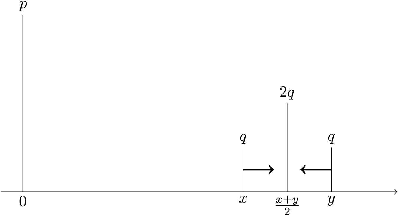
Axiom 2. For any with , any with , and any ,
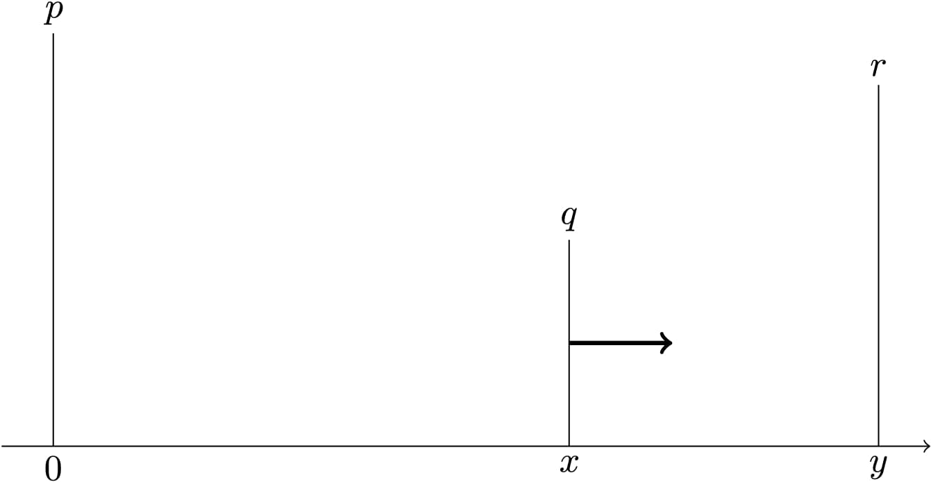
Axiom 3. For any , any with , and any ,
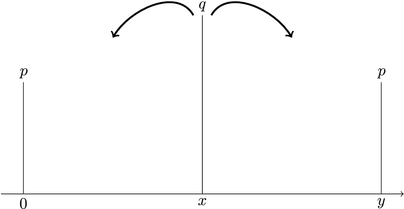
In addition to these foundational axioms, we also include a property proposed by Professor Jesús Aranda. Derived as an intermediate point from Axiom 3, this property—temporarily referred to as Property 1—captures an additional nuance in the behavior of polarization measures.
Property 1. For any , any with and , and any ,
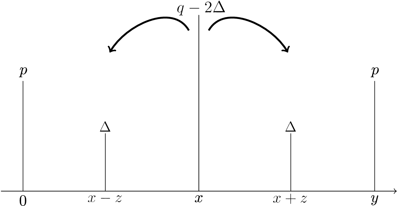
Our goal is to analyze how different measures from the literature align with these fundamental axioms and with Property 1. This analysis will provide insights into the theoretical underpinnings of each measure and their ability to capture the essential properties of polarization as formalized by Esteban and Ray, as well as the additional nuance proposed by Professor Aranda.
For the moment, we conducted a preliminary study using our set of opinion distributions. In this study, each polarization measure (namely MEC, EMD, ER, Shannon, VanDerEijk, and BiPol) was evaluated against several theoretical conditions—namely, Condition H, Axiom 1, Axiom 2, Axiom 3, and Property 1. (For a detailed implementation, please refer to our Colab Notebook
The framework of the test is summarized as follows:
def test_all_measures():
    measures = {
        'MEC': MECNormalized(2, 1.15),
        'EMD': EMDPol(),
        'ER': EstebanRay(0.8),
        'Shannon': ShannonPol(),
        'VanDerEijk': VanDerEijkPol(),
        'BiPol': BiPol()
    }
    results = {}
    for name, measure in measures.items():
        results[name] = {
            'Axiom 1': test_axiom1(measure)['passes'],
            'Axiom 2': test_axiom2(measure)['passes'],
            'Axiom 3': test_axiom3(measure)['passes'],
            'Property 1': test_property1(measure)['passes']
        }
    df_results = pd.DataFrame(results).T
    return results
Below is the summary table of the test results:
| Measure | Axiom 1 | Axiom 2 | Axiom 3 | Property 1 |
|---|---|---|---|---|
| ✓ | ✓ | ✓ | ✓ | |
| ✗ | ✓ | ✓ | ✓ | |
| ✓ | ✓ | ✓ | ✗ | |
| ✗ | ✓ | ✓ | ✓ | |
| ✓ | ✓ | ✓ | ✓ | |
| ✗ | ✓ | ✓ | ✓ |
Although this study is preliminary, it already provides counterexamples that show some measures do not fully satisfy the axioms. For instance, fails Axiom 1 since its polarization value remains when comparing the original distribution with the modified distribution . Similarly, violates Property 1 as its value drops from to when the distribution is altered to under parameters , , , and ; likewise, exhibits an Axiom 1 failure (from to ), and does not preserve the order of ties. In contrast, satisfies all the axioms and Property 1—aligning with expert opinion at 88%—whereas , despite meeting the axioms, corresponds to experts only 67% of the time. Proofs for ’s compliance are pending publication, and future studies will investigate these properties in more depth, including Condition H.
Threshold Analysis for Polarization Classification
A preliminary analysis was performed to establish thresholds for classifying polarization measure values into low, medium, and high categories. In this study, three measures were considered: , , and . For each measure, thresholds were derived using multiple percentile-based schemes. In particular, the 33rd/66th split, the 25th/50th/75th split, and the 20th/40th/60th/80th split were applied to the computed values across all distributions.
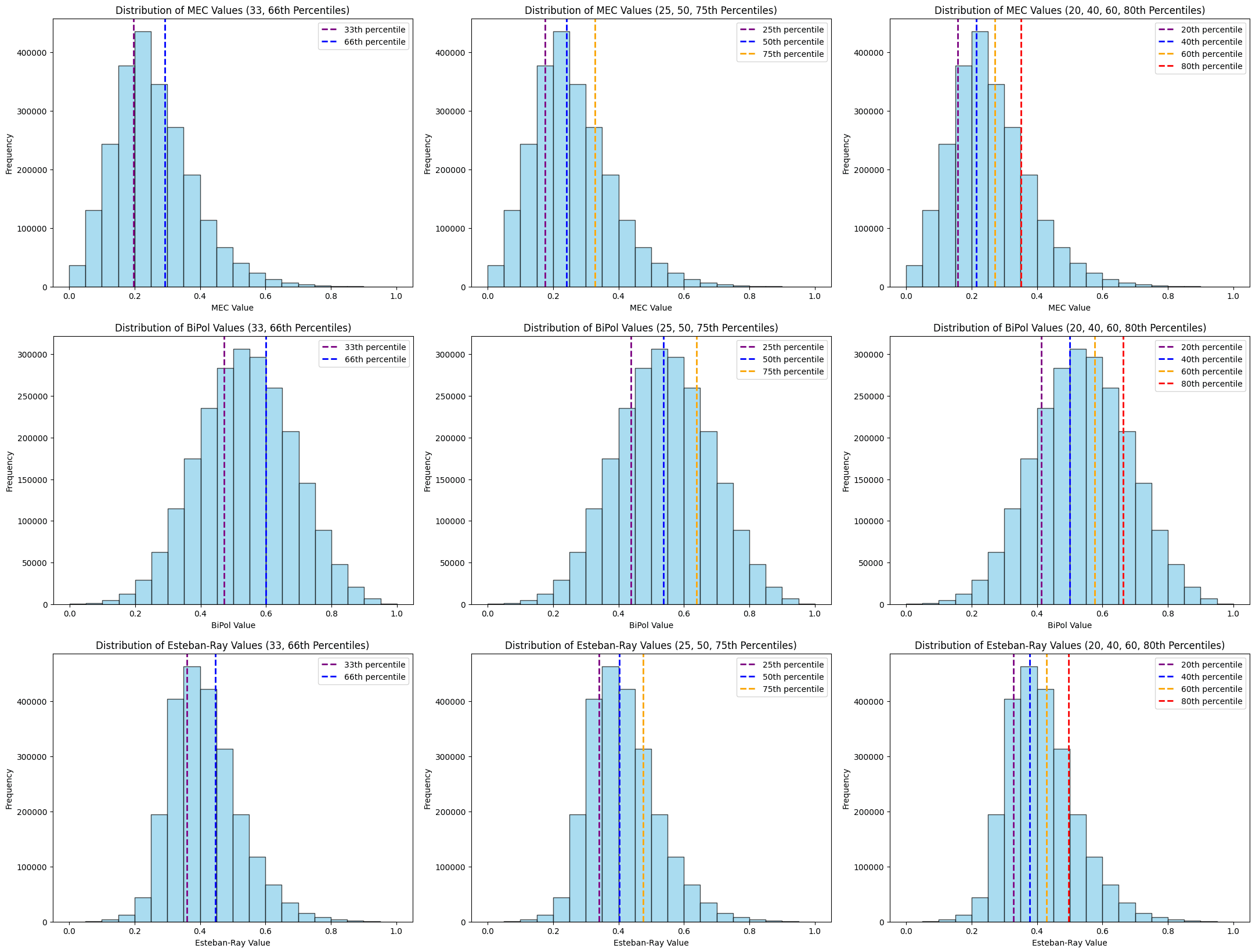
The image illustrates the distribution of polarization values obtained for three measures. The first row corresponds to , the second row to , and the third row to . In this context, the first set of results in the table (the first "column" of splits) represents the 33rd/66th split, the next set corresponds to the 25th/50th/75th split, and the final set pertains to the 20th/40th/60th/80th split. This arrangement allows us to compare how the thresholds, descriptive statistics, and counts change with each percentile partitioning strategy.
Below is the table summarizing these results (excluding the value ranges):
| Measure & Scheme | Thresholds | Descriptive Stats | Counts |
|---|---|---|---|
| MEC, 33rd/66th | 0.1971 / 0.2922 | [0.0000, 0.2574, 0.2408, 1.0000] | (758910, 758909, 781907) |
| BiPol, 33rd/66th | 0.4726 / 0.5994 | [0.0000, 0.5379, 0.5376, 1.0000] | (758979, 758859, 781888) |
| EstebanRay, 33rd/66th | 0.3609 / 0.4466 | [0.0000, 0.4157, 0.4031, 1.0000] | (758910, 758909, 781907) |
| MEC, 25th/50th/75th | 0.1747 / 0.2408 / 0.3274 | [0.0000, 0.2574, 0.2408, 1.0000] | (574932, 574931, 574931, 574932) |
| BiPol, 25th/50th/75th | 0.4380 / 0.5376 / 0.6383 | [0.0000, 0.5379, 0.5376, 1.0000] | (575029, 574883, 574967, 574847) |
| EstebanRay, 25th/50th/75th | 0.3407 / 0.4031 / 0.4761 | [0.0000, 0.4157, 0.4031, 1.0000] | (574932, 574931, 574931, 574932) |
| MEC, 20th/40th/60th/80th | 0.1581 / 0.2141 / 0.2716 / 0.3503 | [0.0000, 0.2574, 0.2408, 1.0000] | (459946, 459945, 459945, 459945, 459945) |
| BiPol, 20th/40th/60th/80th | 0.4140 / 0.5000 / 0.5756 / 0.6627 | [0.0000, 0.5379, 0.5376, 1.0000] | (460296, 459784, 460139, 459566, 459941) |
| EstebanRay, 20th/40th/60th/80th | 0.3275 / 0.3781 / 0.4295 / 0.4965 | [0.0000, 0.4157, 0.4031, 1.0000] | (459946, 459945, 459945, 459945, 459945) |
In this table, the "Descriptive Stats" column follows the format [Min, Mean, Median, Max]. The "Counts" column indicates the number of distributions falling within each category defined by the respective thresholds. For instance, under a 33rd/66th split, there are three categories (Low, Medium, High), whereas the 25th/50th/75th and 20th/40th/60th/80th splits yield four and five categories, respectively.
The detailed percentile analyses have provided valuable insight into the overall dispersion and central tendency of each measure’s distribution. However, they also reveal certain limitations inherent in a uniform, percentile-based approach. While percentiles offer a useful general intuition, they impose rigid, pre-determined divisions on the data that may not capture the natural clustering or subtle nuances present in the distribution of polarization values. This is particularly evident for measures such as , , and , where extreme polarization values tend to be concentrated within a much narrower interval than a uniform split would suggest.
These disadvantages motivated us to explore an alternative approach using the -means clustering algorithm. The -means algorithm is a well-established iterative refinement technique that partitions data into clusters. It begins with an initial set of means, denoted by , and then alternates between two key steps. In the assignment step, each observation is allocated to the cluster with the nearest mean based on the least squared Euclidean distance. This can be mathematically expressed for iteration as
where each observation is assigned exclusively to one cluster, even if it might be equidistant from more than one mean. Following this, the update step recalculates the means (or centroids) for each cluster using the formula
With each iteration, the algorithm minimizes the within-cluster sum of squares (WCSS), ensuring a nonnegative, monotonically decreasing sequence that leads to convergence, although not necessarily to the global optimum. This iterative process, often referred to as Lloyd's algorithm or simply as -means, adapts to the intrinsic structure of the data by uncovering natural groupings that a uniform percentile-based approach might miss.
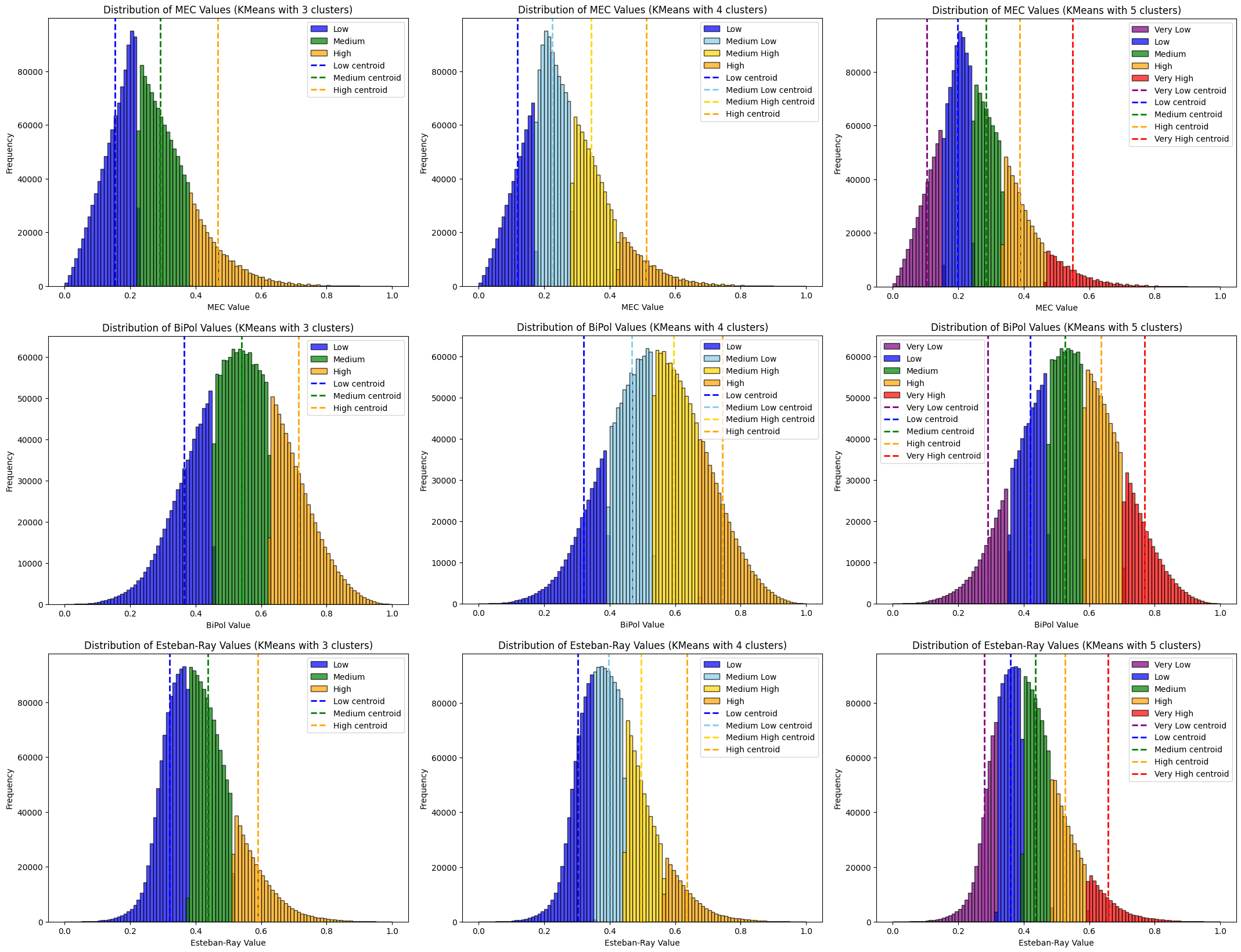
The k-means clustering results image shows how polarization values naturally group for three measures. The first row corresponds to , the second to , and the third to . Within each row, the first column represents the case when , the second when , and the third when . This presentation allows us to observe how the grouping structure evolves as the number of clusters increases. The counts of observations assigned to each cluster, presented in the same format as in the percentile analysis, provide additional insight into the distribution of values across the clusters. The table below summarizes these results.
| Measure (k) | Cluster Centroids | Counts | Value Ranges |
|---|---|---|---|
| MEC (k=3) | [0.1546, 0.2919, 0.4683] | (1002929, 960752, 336045) | [0.0000, 0.2233] / [0.2233, 0.3801] / [0.3801, 1.0000] |
| BiPol (k=3) | [0.3652, 0.5398, 0.7137] | (649188, 1016983, 633555) | [0.0000, 0.4525] / [0.4526, 0.6267] / [0.6268, 1.0000] |
| Esteban-Ray (k=3) | [0.3202, 0.4380, 0.5902] | (928943, 993213, 377570) | [0.0000, 0.3791] / [0.3791, 0.5141] / [0.5141, 1.0000] |
| MEC (k=4) | [0.1182, 0.2255, 0.3428, 0.5114] | (554166, 911036, 633659, 200865) | [0.0000, 0.1718] / [0.1718, 0.2841] / [0.2841, 0.4271] / [0.4271, 1.0000] |
| BiPol (k=4) | [0.3208, 0.4672, 0.5963, 0.7442] | (376399, 736586, 760015, 426726) | [0.0000, 0.3940] / [0.3941, 0.5317] / [0.5318, 0.6702] / [0.6703, 1.0000] |
| Esteban-Ray (k=4) | [0.3027, 0.3975, 0.4959, 0.6361] | (659528, 859091, 578046, 203061) | [0.0000, 0.3501] / [0.3501, 0.4467] / [0.4467, 0.5660] / [0.5660, 1.0000] |
| MEC (k=5) | [0.1040, 0.1987, 0.2855, 0.3883, 0.5495] | (417349, 742128, 614763, 398368, 127118) | [0.0000, 0.1513] / [0.1513, 0.2421] / [0.2421, 0.3369] / [0.3369, 0.4689] / [0.4689, 1.0000] |
| BiPol (k=5) | [0.2895, 0.4191, 0.5269, 0.6364, 0.7686] | (237904, 523153, 654893, 581750, 302026) | [0.0000, 0.3543] / [0.3544, 0.4730] / [0.4731, 0.5816] / [0.5817, 0.7024] / [0.7025, 1.0000] |
| Esteban-Ray (k=5) | [0.2803, 0.3588, 0.4358, 0.5259, 0.6582] | (395345, 701921, 656490, 401449, 144521) | [0.0000, 0.3196] / [0.3196, 0.3973] / [0.3973, 0.4809] / [0.4809, 0.5921] / [0.5921, 1.0000] |
In our study, the application of -means clustering confirmed that extreme polarization values are relatively rare and tend to cluster within a narrow interval. This finding highlights the advantage of using -means to refine threshold determination, as it more accurately reflects the underlying distribution of the polarization measures. For future studies, we plan to examine the correlation among these measures within the identified clusters, which may reveal further insights into how different indices capture the same underlying phenomena of opinion divergence. Overall, our integrated approach—combining theoretical modeling, extensive computational analysis, and expert validation—provides a robust framework for understanding and classifying polarization. By bridging theoretical rigor with empirical evidence, this work lays the groundwork for more nuanced and reliable assessments of polarization in complex social systems, and it opens promising avenues for future research in the field.